Notice

Recent Posts

Recent Comments

Link

« 2024/12 »
일	월	화	수	목	금	토
1	2	3	4	5	6	7
8	9	10	11	12	13	14
15	16	17	18	19	20	21
22	23	24	25	26	27	28
29	30	31

Tags more

Archives

Today

Total

관리 메뉴

獨斷論

27 Survival analysis 본문

과학과 기술/R 통계

27 Survival analysis

부르칸 2023. 3. 28. 02:54

27 Survival analysis

27.1 Overview

Survival analysis focuses on describing for a given individual or group of individuals, a defined point of event called the failure (occurrence of a disease, cure from a disease, death, relapse after response to treatment…) that occurs after a period of time called failure time (or follow-up time in cohort/population-based studies) during which individuals are observed. To determine the failure time, it is then necessary to define a time of origin (that can be the inclusion date, the date of diagnosis…).

The target of inference for survival analysis is then the time between an origin and an event. In current medical research, it is widely used in clinical studies to assess the effect of a treatment for instance, or in cancer epidemiology to assess a large variety of cancer survival measures.

It is usually expressed through the survival probability which is the probability that the event of interest has not occurred by a duration t.

Censoring: Censoring occurs when at the end of follow-up, some of the individuals have not had the event of interest, and thus their true time to event is unknown. We will mostly focus on right censoring here but for more details on censoring and survival analysis in general, you can see references.

27.2 Preparation

Load packages

To run survival analyses in R, one the most widely used package is the survival package. We first install it and then load it as well as the other packages that will be used in this section:

In this handbook we emphasize p_load() from pacman, which installs the package if necessary and loads it for use. You can also load installed packages with library() from base R. See the page on R basics for more information on R packages.

This page explores survival analyses using the linelist used in most of the previous pages and on which we apply some changes to have a proper survival data.

Import dataset

We import the dataset of cases from a simulated Ebola epidemic. If you want to follow along, click to download the “clean” linelist (as .rds file). Import data with the import() function from the rio package (it handles many file types like .xlsx, .csv, .rds - see the Import and export page for details).

# import linelist
linelist_case_data <- rio::import("linelist_cleaned.rds")

Data management and transformation

In short, survival data can be described as having the following three characteristics:

the dependent variable or response is the waiting time until the occurrence of a well-defined event,
observations are censored, in the sense that for some units the event of interest has not occurred at the time the data are analyzed, and
there are predictors or explanatory variables whose effect on the waiting time we wish to assess or control.

Thus, we will create different variables needed to respect that structure and run the survival analysis.

We define:

a new data frame linelist_surv for this analysis
our event of interest as being “death” (hence our survival probability will be the probability of being alive after a certain time after the time of origin),
the follow-up time (futime) as the time between the time of onset and the time of outcome in days,
censored patients as those who recovered or for whom the final outcome is not known ie the event “death” was not observed (event=0).

CAUTION: Since in a real cohort study, the information on the time of origin and the end of the follow-up is known given individuals are observed, we will remove observations where the date of onset or the date of outcome is unknown. Also the cases where the date of onset is later than the date of outcome will be removed since they are considered as wrong.

TIP: Given that filtering to greater than (>) or less than (<) a date can remove rows with missing values, applying the filter on the wrong dates will also remove the rows with missing dates.

We then use case_when() to create a column age_cat_small in which there are only 3 age categories.

#create a new data called linelist_surv from the linelist_case_data

linelist_surv <-  linelist_case_data %>% 
     
  dplyr::filter(
       # remove observations with wrong or missing dates of onset or date of outcome
       date_outcome > date_onset) %>% 
  
  dplyr::mutate(
       # create the event var which is 1 if the patient died and 0 if he was right censored
       event = ifelse(is.na(outcome) | outcome == "Recover", 0, 1), 
    
       # create the var on the follow-up time in days
       futime = as.double(date_outcome - date_onset), 
    
       # create a new age category variable with only 3 strata levels
       age_cat_small = dplyr::case_when( 
            age_years < 5  ~ "0-4",
            age_years >= 5 & age_years < 20 ~ "5-19",
            age_years >= 20   ~ "20+"),
       
       # previous step created age_cat_small var as character.
       # now convert it to factor and specify the levels.
       # Note that the NA values remain NA's and are not put in a level "unknown" for example,
       # since in the next analyses they have to be removed.
       age_cat_small = fct_relevel(age_cat_small, "0-4", "5-19", "20+")
       )

TIP: We can verify the new columns we have created by doing a summary on the futime and a cross-tabulation between event and outcome from which it was created. Besides this verification it is a good habit to communicate the median follow-up time when interpreting survival analysis results.

summary(linelist_surv$futime)

##    Min. 1st Qu.  Median    Mean 3rd Qu.    Max. 
##    1.00    6.00   10.00   11.98   16.00   64.00

# cross tabulate the new event var and the outcome var from which it was created
# to make sure the code did what it was intended to
linelist_surv %>% 
  tabyl(outcome, event)

##  outcome    0    1
##    Death    0 1952
##  Recover 1547    0
##     <NA> 1040    0

Now we cross-tabulate the new age_cat_small var and the old age_cat col to ensure correct assingments

linelist_surv %>% 
  tabyl(age_cat_small, age_cat)

##  age_cat_small 0-4 5-9 10-14 15-19 20-29 30-49 50-69 70+ NA_
##            0-4 834   0     0     0     0     0     0   0   0
##           5-19   0 852   717   575     0     0     0   0   0
##            20+   0   0     0     0   862   554    69   5   0
##           <NA>   0   0     0     0     0     0     0   0  71

Now we review the 10 first observations of the linelist_surv data looking at specific variables (including those newly created).

linelist_surv %>% 
  select(case_id, age_cat_small, date_onset, date_outcome, outcome, event, futime) %>% 
  head(10)

##    case_id age_cat_small date_onset date_outcome outcome event futime
## 1   8689b7           0-4 2014-05-13   2014-05-18 Recover     0      5
## 2   11f8ea           20+ 2014-05-16   2014-05-30 Recover     0     14
## 3   893f25           0-4 2014-05-21   2014-05-29 Recover     0      8
## 4   be99c8          5-19 2014-05-22   2014-05-24 Recover     0      2
## 5   07e3e8          5-19 2014-05-27   2014-06-01 Recover     0      5
## 6   369449           0-4 2014-06-02   2014-06-07   Death     1      5
## 7   f393b4           20+ 2014-06-05   2014-06-18 Recover     0     13
## 8   1389ca           20+ 2014-06-05   2014-06-09   Death     1      4
## 9   2978ac          5-19 2014-06-06   2014-06-15   Death     1      9
## 10  fc15ef          5-19 2014-06-16   2014-07-09 Recover     0     23

We can also cross-tabulate the columns age_cat_small and gender to have more details on the distribution of this new column by gender. We use tabyl() and the adorn functions from janitor as described in the Descriptive tables page.

linelist_surv %>% 
  tabyl(gender, age_cat_small, show_na = F) %>% 
  adorn_totals(where = "both") %>% 
  adorn_percentages() %>% 
  adorn_pct_formatting() %>% 
  adorn_ns(position = "front")

##  gender         0-4         5-19          20+         Total
##       f 482 (22.4%) 1184 (54.9%)  490 (22.7%) 2156 (100.0%)
##       m 325 (15.0%)  880 (40.6%)  960 (44.3%) 2165 (100.0%)
##   Total 807 (18.7%) 2064 (47.8%) 1450 (33.6%) 4321 (100.0%)

27.3 Basics of survival analysis

Building a surv-type object

We will first use Surv() from survival to build a survival object from the follow-up time and event columns.

The result of such a step is to produce an object of type Surv that condenses the time information and whether the event of interest (death) was observed. This object will ultimately be used in the right-hand side of subsequent model formulae (see documentation).

# Use Suv() syntax for right-censored data
survobj <- Surv(time = linelist_surv$futime,
                event = linelist_surv$event)

To review, here are the first 10 rows of the linelist_surv data, viewing only some important columns.

linelist_surv %>% 
  select(case_id, date_onset, date_outcome, futime, outcome, event) %>% 
  head(10)

##    case_id date_onset date_outcome futime outcome event
## 1   8689b7 2014-05-13   2014-05-18      5 Recover     0
## 2   11f8ea 2014-05-16   2014-05-30     14 Recover     0
## 3   893f25 2014-05-21   2014-05-29      8 Recover     0
## 4   be99c8 2014-05-22   2014-05-24      2 Recover     0
## 5   07e3e8 2014-05-27   2014-06-01      5 Recover     0
## 6   369449 2014-06-02   2014-06-07      5   Death     1
## 7   f393b4 2014-06-05   2014-06-18     13 Recover     0
## 8   1389ca 2014-06-05   2014-06-09      4   Death     1
## 9   2978ac 2014-06-06   2014-06-15      9   Death     1
## 10  fc15ef 2014-06-16   2014-07-09     23 Recover     0

And here are the first 10 elements of survobj. It prints as essentially a vector of follow-up time, with “+” to represent if an observation was right-censored. See how the numbers align above and below.

#print the 50 first elements of the vector to see how it presents
head(survobj, 10)

##  [1]  5+ 14+  8+  2+  5+  5  13+  4   9  23+

Running initial analyses

We then start our analysis using the survfit() function to produce a survfit object, which fits the default calculations for Kaplan Meier (KM) estimates of the overall (marginal) survival curve, which are in fact a step function with jumps at observed event times. The final survfit object contains one or more survival curves and is created using the Surv object as a response variable in the model formula.

NOTE: The Kaplan-Meier estimate is a nonparametric maximum likelihood estimate (MLE) of the survival function. . (see resources for more information).

The summary of this survfit object will give what is called a life table. For each time step of the follow-up (time) where an event happened (in ascending order):

the number of people who were at risk of developing the event (people who did not have the event yet nor were censored: n.risk)
those who did develop the event (n.event)
and from the above: the probability of not developing the event (probability of not dying, or of surviving past that specific time)
finally, the standard error and the confidence interval for that probability are derived and displayed

We fit the KM estimates using the formula where the previously Surv object “survobj” is the response variable. “~ 1” precises we run the model for the overall survival.

# fit the KM estimates using a formula where the Surv object "survobj" is the response variable.
# "~ 1" signifies that we run the model for the overall survival  
linelistsurv_fit <-  survival::survfit(survobj ~ 1)

#print its summary for more details
summary(linelistsurv_fit)

## Call: survfit(formula = survobj ~ 1)
## 
##  time n.risk n.event survival std.err lower 95% CI upper 95% CI
##     1   4539      30    0.993 0.00120        0.991        0.996
##     2   4500      69    0.978 0.00217        0.974        0.982
##     3   4394     149    0.945 0.00340        0.938        0.952
##     4   4176     194    0.901 0.00447        0.892        0.910
##     5   3899     214    0.852 0.00535        0.841        0.862
##     6   3592     210    0.802 0.00604        0.790        0.814
##     7   3223     179    0.757 0.00656        0.745        0.770
##     8   2899     167    0.714 0.00700        0.700        0.728
##     9   2593     145    0.674 0.00735        0.660        0.688
##    10   2311     109    0.642 0.00761        0.627        0.657
##    11   2081     119    0.605 0.00788        0.590        0.621
##    12   1843      89    0.576 0.00809        0.560        0.592
##    13   1608      55    0.556 0.00823        0.540        0.573
##    14   1448      43    0.540 0.00837        0.524        0.556
##    15   1296      31    0.527 0.00848        0.511        0.544
##    16   1152      48    0.505 0.00870        0.488        0.522
##    17   1002      29    0.490 0.00886        0.473        0.508
##    18    898      21    0.479 0.00900        0.462        0.497
##    19    798       7    0.475 0.00906        0.457        0.493
##    20    705       4    0.472 0.00911        0.454        0.490
##    21    626      13    0.462 0.00932        0.444        0.481
##    22    546       8    0.455 0.00948        0.437        0.474
##    23    481       5    0.451 0.00962        0.432        0.470
##    24    436       4    0.447 0.00975        0.428        0.466
##    25    378       4    0.442 0.00993        0.423        0.462
##    26    336       3    0.438 0.01010        0.419        0.458
##    27    297       1    0.436 0.01017        0.417        0.457
##    29    235       1    0.435 0.01030        0.415        0.455
##    38     73       1    0.429 0.01175        0.406        0.452

While using summary() we can add the option times and specify certain times at which we want to see the survival information

#print its summary at specific times
summary(linelistsurv_fit, times = c(5,10,20,30,60))

## Call: survfit(formula = survobj ~ 1)
## 
##  time n.risk n.event survival std.err lower 95% CI upper 95% CI
##     5   3899     656    0.852 0.00535        0.841        0.862
##    10   2311     810    0.642 0.00761        0.627        0.657
##    20    705     446    0.472 0.00911        0.454        0.490
##    30    210      39    0.435 0.01030        0.415        0.455
##    60      2       1    0.429 0.01175        0.406        0.452

We can also use the print() function. The print.rmean = TRUE argument is used to obtain the mean survival time and its standard error (se).

NOTE: The restricted mean survival time (RMST) is a specific survival measure more and more used in cancer survival analysis and which is often defined as the area under the survival curve, given we observe patients up to restricted time T (more details in Resources section).

# print linelistsurv_fit object with mean survival time and its se. 
print(linelistsurv_fit, print.rmean = TRUE)

## Call: survfit(formula = survobj ~ 1)
## 
##         n events rmean* se(rmean) median 0.95LCL 0.95UCL
## [1,] 4539   1952   33.1     0.539     17      16      18
##     * restricted mean with upper limit =  64

TIP: We can create the surv object directly in the survfit() function and save a line of code. This will then look like: linelistsurv_quick <- survfit(Surv(futime, event) ~ 1, data=linelist_surv).

Cumulative hazard

Besides the summary() function, we can also use the str() function that gives more details on the structure of the survfit() object. It is a list of 16 elements.

Among these elements is an important one: cumhaz, which is a numeric vector. This could be plotted to allow show the cumulative hazard, with the hazard being the instantaneous rate of event occurrence (see references).

str(linelistsurv_fit)

## List of 16
##  $ n        : int 4539
##  $ time     : num [1:59] 1 2 3 4 5 6 7 8 9 10 ...
##  $ n.risk   : num [1:59] 4539 4500 4394 4176 3899 ...
##  $ n.event  : num [1:59] 30 69 149 194 214 210 179 167 145 109 ...
##  $ n.censor : num [1:59] 9 37 69 83 93 159 145 139 137 121 ...
##  $ surv     : num [1:59] 0.993 0.978 0.945 0.901 0.852 ...
##  $ std.err  : num [1:59] 0.00121 0.00222 0.00359 0.00496 0.00628 ...
##  $ cumhaz   : num [1:59] 0.00661 0.02194 0.05585 0.10231 0.15719 ...
##  $ std.chaz : num [1:59] 0.00121 0.00221 0.00355 0.00487 0.00615 ...
##  $ type     : chr "right"
##  $ logse    : logi TRUE
##  $ conf.int : num 0.95
##  $ conf.type: chr "log"
##  $ lower    : num [1:59] 0.991 0.974 0.938 0.892 0.841 ...
##  $ upper    : num [1:59] 0.996 0.982 0.952 0.91 0.862 ...
##  $ call     : language survfit(formula = survobj ~ 1)
##  - attr(*, "class")= chr "survfit"

Plotting Kaplan-Meir curves

Once the KM estimates are fitted, we can visualize the probability of being alive through a given time using the basic plot() function that draws the “Kaplan-Meier curve”. In other words, the curve below is a conventional illustration of the survival experience in the whole patient group.

We can quickly verify the follow-up time min and max on the curve.

An easy way to interpret is to say that at time zero, all the participants are still alive and survival probability is then 100%. This probability decreases over time as patients die. The proportion of participants surviving past 60 days of follow-up is around 40%.

plot(linelistsurv_fit, 
     xlab = "Days of follow-up",    # x-axis label
     ylab="Survival Probability",   # y-axis label
     main= "Overall survival curve" # figure title
     )

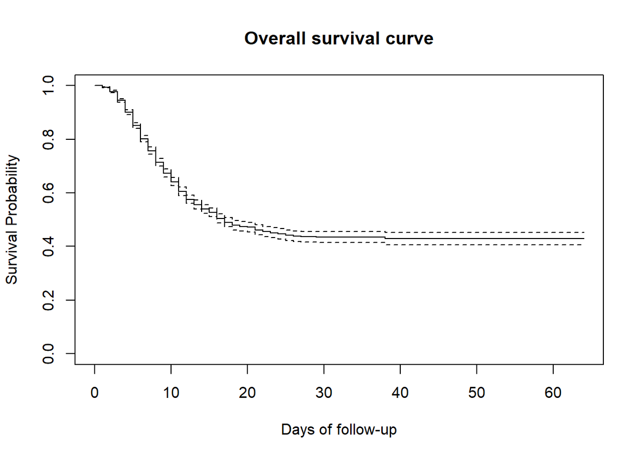
The confidence interval of the KM survival estimates are also plotted by default and can be dismissed by adding the option conf.int = FALSE to the plot() command.

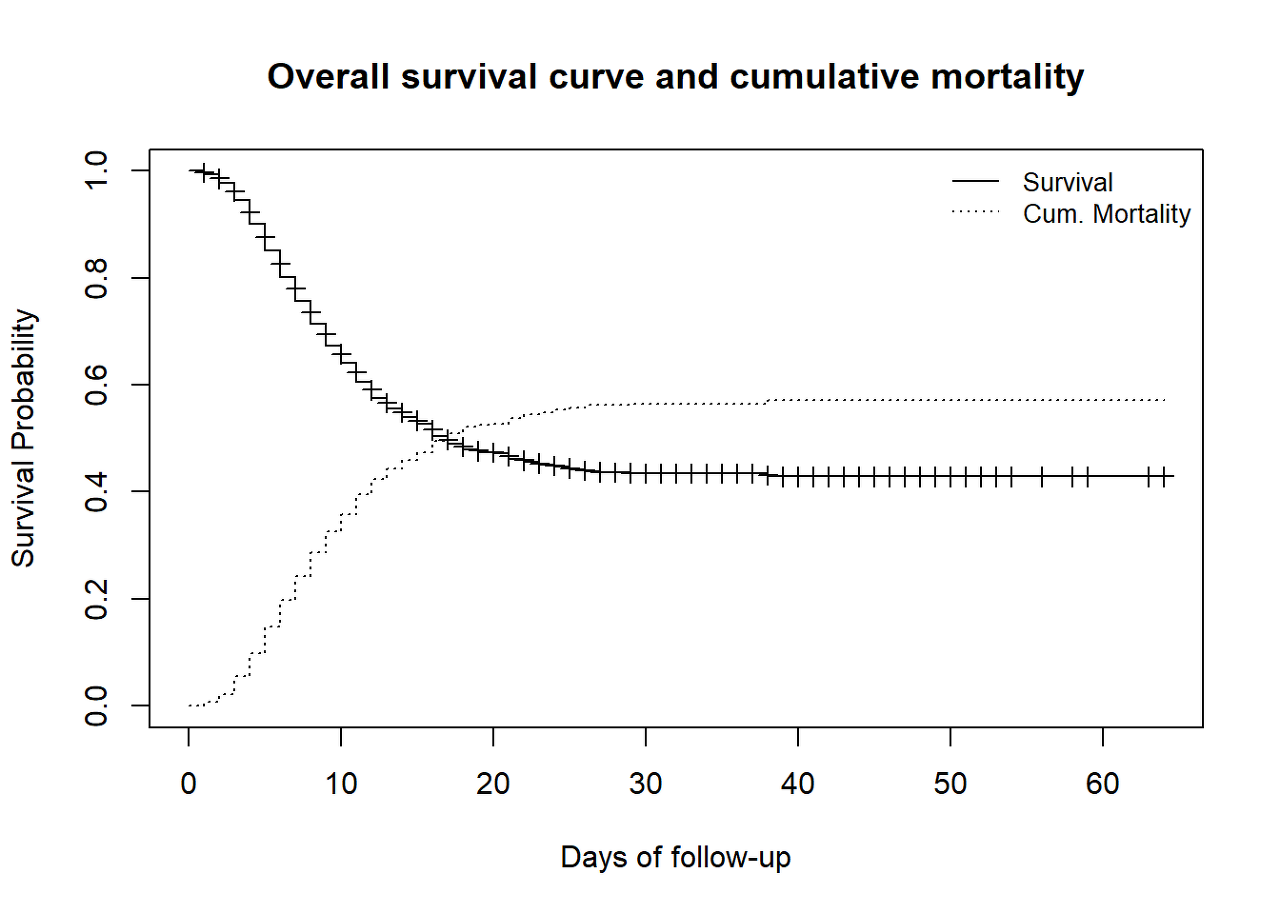
Since the event of interest is “death”, drawing a curve describing the complements of the survival proportions will lead to drawing the cumulative mortality proportions. This can be done with lines(), which adds information to an existing plot.

# original plot
plot(
  linelistsurv_fit,
  xlab = "Days of follow-up",       
  ylab = "Survival Probability",       
  mark.time = TRUE,              # mark events on the curve: a "+" is printed at every event
  conf.int = FALSE,              # do not plot the confidence interval
  main = "Overall survival curve and cumulative mortality"
  )

# draw an additional curve to the previous plot
lines(
  linelistsurv_fit,
  lty = 3,             # use different line type for clarity
  fun = "event",       # draw the cumulative events instead of the survival 
  mark.time = FALSE,
  conf.int = FALSE
  )

# add a legend to the plot
legend(
  "topright",                               # position of legend
  legend = c("Survival", "Cum. Mortality"), # legend text 
  lty = c(1, 3),                            # line types to use in the legend
  cex = .85,                                # parametes that defines size of legend text
  bty = "n"                                 # no box type to be drawn for the legend
  )

27.4 Comparison of survival curves

To compare the survival within different groups of our observed participants or patients, we might need to first look at their respective survival curves and then run tests to evaluate the difference between independent groups. This comparison can concern groups based on gender, age, treatment, comorbidity…

Log rank test

The log rank test is a popular test that compares the entire survival experience between two or more independent groups and can be thought of as a test of whether the survival curves are identical (overlapping) or not (null hypothesis of no difference in survival between the groups). The survdiff() function of the survival package allows running the log-rank test when we specify rho = 0 (which is the default). The test results gives a chi-square statistic along with a p-value since the log rank statistic is approximately distributed as a chi-square test statistic.

We first try to compare the survival curves by gender group. For this, we first try to visualize it (check whether the two survival curves are overlapping). A new survfit object will be created with a slightly different formula. Then the survdiff object will be created.

By supplying ~ gender as the right side of the formula, we no longer plot the overall survival but instead by gender.

# create the new survfit object based on gender
linelistsurv_fit_sex <-  survfit(Surv(futime, event) ~ gender, data = linelist_surv)

Now we can plot the survival curves by gender. Have a look at the order of the strata levels in the gender column before defining your colors and legend.

# set colors
col_sex <- c("lightgreen", "darkgreen")

# create plot
plot(
  linelistsurv_fit_sex,
  col = col_sex,
  xlab = "Days of follow-up",
  ylab = "Survival Probability")

# add legend
legend(
  "topright",
  legend = c("Female","Male"),
  col = col_sex,
  lty = 1,
  cex = .9,
  bty = "n")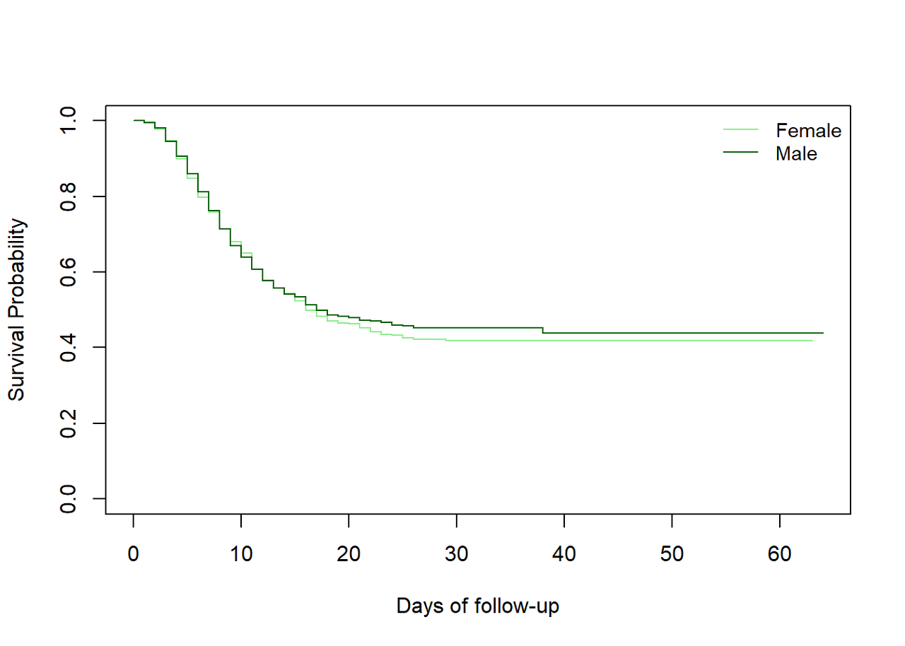

And now we can compute the test of the difference between the survival curves using survdiff()

#compute the test of the difference between the survival curves
survival::survdiff(
  Surv(futime, event) ~ gender, 
  data = linelist_surv
  )

## Call:
## survival::survdiff(formula = Surv(futime, event) ~ gender, data = linelist_surv)
## 
## n=4321, 218 observations deleted due to missingness.
## 
##             N Observed Expected (O-E)^2/E (O-E)^2/V
## gender=f 2156      924      909     0.255     0.524
## gender=m 2165      929      944     0.245     0.524
## 
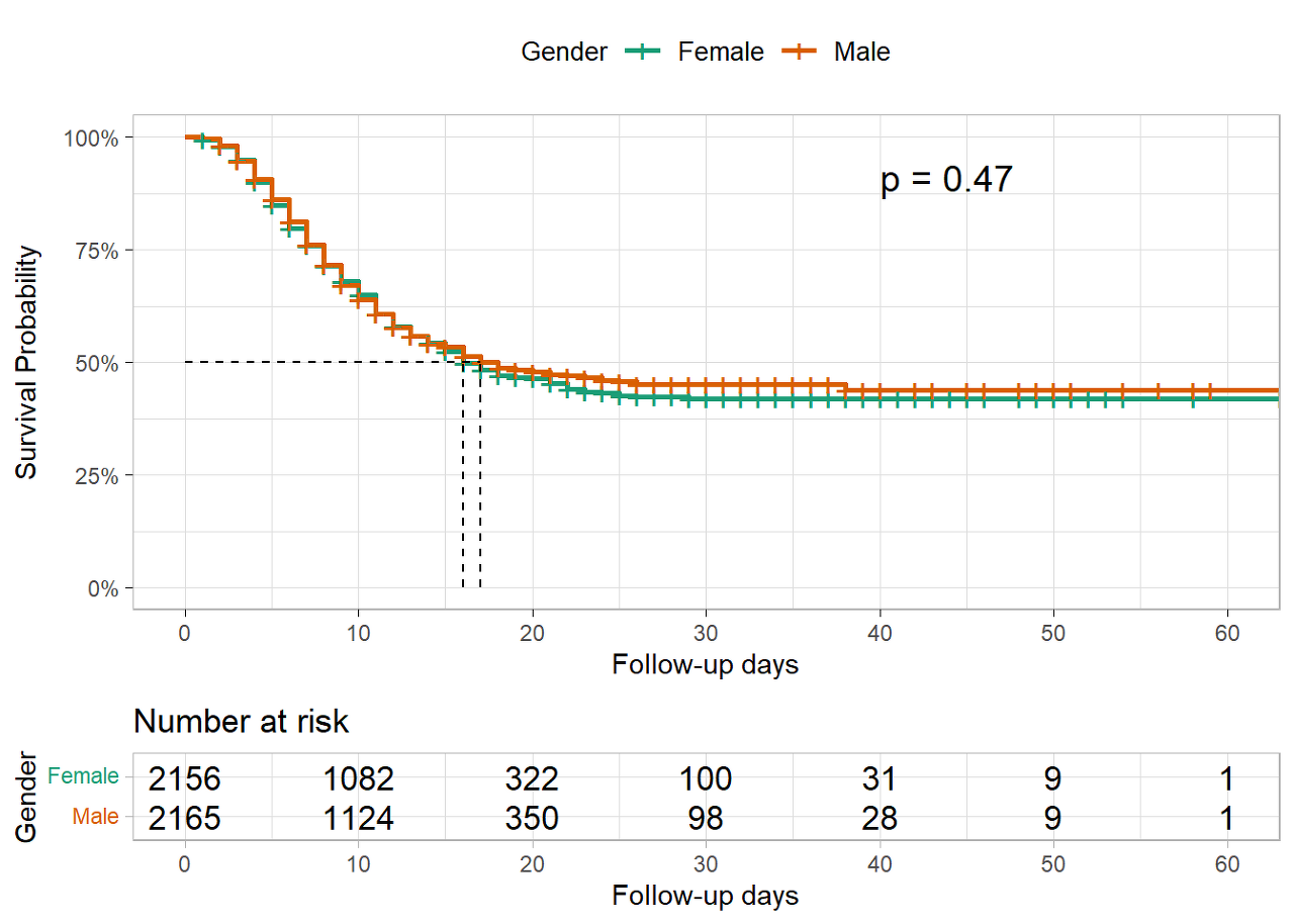
##  Chisq= 0.5  on 1 degrees of freedom, p= 0.5

We see that the survival curve for women and the one for men overlap and the log-rank test does not give evidence of a survival difference between women and men.

Some other R packages allow illustrating survival curves for different groups and testing the difference all at once. Using the ggsurvplot() function from the survminer package, we can also include in our curve the printed risk tables for each group, as well the p-value from the log-rank test.

CAUTION: survminer functions require that you specify the survival object and again specify the data used to fit the survival object. Remember to do this to avoid non-specific error messages.

survminer::ggsurvplot(
    linelistsurv_fit_sex, 
    data = linelist_surv,          # again specify the data used to fit linelistsurv_fit_sex 
    conf.int = FALSE,              # do not show confidence interval of KM estimates
    surv.scale = "percent",        # present probabilities in the y axis in %
    break.time.by = 10,            # present the time axis with an increment of 10 days
    xlab = "Follow-up days",
    ylab = "Survival Probability",
    pval = T,                      # print p-value of Log-rank test 
    pval.coord = c(40,.91),        # print p-value at these plot coordinates
    risk.table = T,                # print the risk table at bottom 
    legend.title = "Gender",       # legend characteristics
    legend.labs = c("Female","Male"),
    font.legend = 10, 
    palette = "Dark2",             # specify color palette 
    surv.median.line = "hv",       # draw horizontal and vertical lines to the median survivals
    ggtheme = theme_light()        # simplify plot background
)

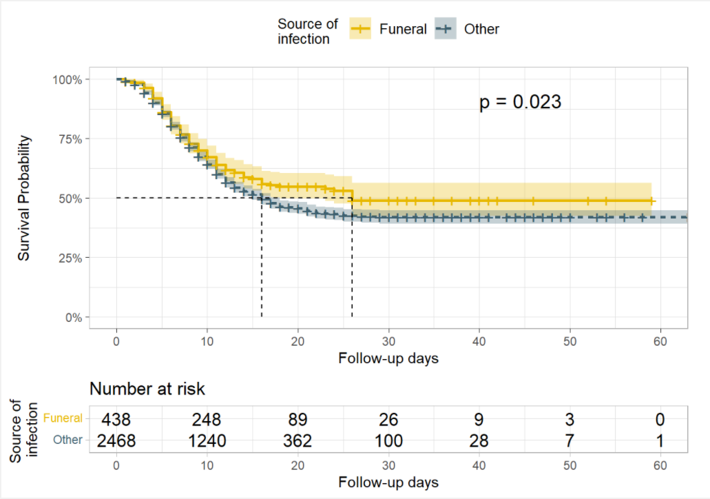
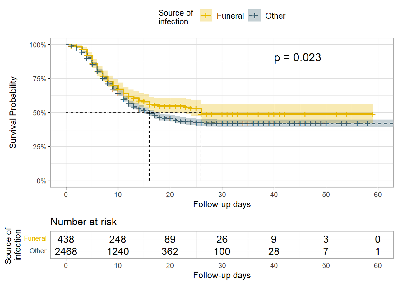
We may also want to test for differences in survival by the source of infection (source of contamination).

In this case, the Log rank test gives enough evidence of a difference in the survival probabilities at alpha= 0.005. The survival probabilities for patients that were infected at funerals are higher than the survival probabilities for patients that got infected in other places, suggesting a survival benefit.

linelistsurv_fit_source <-  survfit(
  Surv(futime, event) ~ source,
  data = linelist_surv
  )

# plot
ggsurvplot( 
  linelistsurv_fit_source,
  data = linelist_surv,
  size = 1, linetype = "strata",   # line types
  conf.int = T,
  surv.scale = "percent",  
  break.time.by = 10, 
  xlab = "Follow-up days",
  ylab= "Survival Probability",
  pval = T,
  pval.coord = c(40,.91),
  risk.table = T,
  legend.title = "Source of \ninfection",
  legend.labs = c("Funeral", "Other"),
  font.legend = 10,
  palette = c("#E7B800","#3E606F"),
  surv.median.line = "hv", 
  ggtheme = theme_light()
)

27.5 Cox regression analysis

Cox proportional hazards regression is one of the most popular regression techniques for survival analysis. Other models can also be used since the Cox model requires important assumptions that need to be verified for an appropriate use such as the proportional hazards assumption: see references.

In a Cox proportional hazards regression model, the measure of effect is the hazard rate (HR), which is the risk of failure (or the risk of death in our example), given that the participant has survived up to a specific time. Usually, we are interested in comparing independent groups with respect to their hazards, and we use a hazard ratio, which is analogous to an odds ratio in the setting of multiple logistic regression analysis. The cox.ph() function from the survival package is used to fit the model. The function cox.zph() from survival package may be used to test the proportional hazards assumption for a Cox regression model fit.

NOTE: A probability must lie in the range 0 to 1. However, the hazard represents the expected number of events per one unit of time.

If the hazard ratio for a predictor is close to 1 then that predictor does not affect survival,
if the HR is less than 1, then the predictor is protective (i.e., associated with improved survival),
and if the HR is greater than 1, then the predictor is associated with increased risk (or decreased survival).

Fitting a Cox model

We can first fit a model to assess the effect of age and gender on the survival. By just printing the model, we have the information on:

the estimated regression coefficients coef which quantifies the association between the predictors and the outcome,
their exponential (for interpretability, exp(coef)) which produces the hazard ratio,
their standard error se(coef),
the z-score: how many standard errors is the estimated coefficient away from 0,
and the p-value: the probability that the estimated coefficient could be 0.

The summary() function applied to the cox model object gives more information, such as the confidence interval of the estimated HR and the different test scores.

The effect of the first covariate gender is presented in the first row. genderm (male) is printed, implying that the first strata level (“f”), i.e the female group, is the reference group for the gender. Thus the interpretation of the test parameter is that of men compared to women. The p-value indicates there was not enough evidence of an effect of the gender on the expected hazard or of an association between gender and all-cause mortality.

The same lack of evidence is noted regarding age-group.

#fitting the cox model
linelistsurv_cox_sexage <-  survival::coxph(
              Surv(futime, event) ~ gender + age_cat_small, 
              data = linelist_surv
              )


#printing the model fitted
linelistsurv_cox_sexage

## Call:
## survival::coxph(formula = Surv(futime, event) ~ gender + age_cat_small, 
##     data = linelist_surv)
## 
##                       coef exp(coef) se(coef)      z     p
## genderm           -0.03149   0.96900  0.04767 -0.661 0.509
## age_cat_small5-19  0.09400   1.09856  0.06454  1.456 0.145
## age_cat_small20+   0.05032   1.05161  0.06953  0.724 0.469
## 
## Likelihood ratio test=2.8  on 3 df, p=0.4243
## n= 4321, number of events= 1853 
##    (218 observations deleted due to missingness)

#summary of the model
summary(linelistsurv_cox_sexage)

## Call:
## survival::coxph(formula = Surv(futime, event) ~ gender + age_cat_small, 
##     data = linelist_surv)
## 
##   n= 4321, number of events= 1853 
##    (218 observations deleted due to missingness)
## 
##                       coef exp(coef) se(coef)      z Pr(>|z|)
## genderm           -0.03149   0.96900  0.04767 -0.661    0.509
## age_cat_small5-19  0.09400   1.09856  0.06454  1.456    0.145
## age_cat_small20+   0.05032   1.05161  0.06953  0.724    0.469
## 
##                   exp(coef) exp(-coef) lower .95 upper .95
## genderm               0.969     1.0320    0.8826     1.064
## age_cat_small5-19     1.099     0.9103    0.9680     1.247
## age_cat_small20+      1.052     0.9509    0.9176     1.205
## 
## Concordance= 0.514  (se = 0.007 )
## Likelihood ratio test= 2.8  on 3 df,   p=0.4
## Wald test            = 2.78  on 3 df,   p=0.4
## Score (logrank) test = 2.78  on 3 df,   p=0.4

It was interesting to run the model and look at the results but a first look to verify whether the proportional hazards assumptions is respected could help saving time.

test_ph_sexage <- survival::cox.zph(linelistsurv_cox_sexage)
test_ph_sexage

##               chisq df    p
## gender        0.454  1 0.50
## age_cat_small 0.838  2 0.66
## GLOBAL        1.399  3 0.71

NOTE: A second argument called method can be specified when computing the cox model, that determines how ties are handled. The default is “efron”, and the other options are “breslow” and “exact”.

In another model we add more risk factors such as the source of infection and the number of days between date of onset and admission. This time, we first verify the proportional hazards assumption before going forward.

In this model, we have included a continuous predictor (days_onset_hosp). In this case we interpret the parameter estimates as the increase in the expected log of the relative hazard for each one unit increase in the predictor, holding other predictors constant. We first verify the proportional hazards assumption.

#fit the model
linelistsurv_cox <-  coxph(
                        Surv(futime, event) ~ gender + age_years+ source + days_onset_hosp,
                        data = linelist_surv
                        )


#test the proportional hazard model
linelistsurv_ph_test <- cox.zph(linelistsurv_cox)
linelistsurv_ph_test

##                    chisq df       p
## gender           0.45062  1    0.50
## age_years        0.00199  1    0.96
## source           1.79622  1    0.18
## days_onset_hosp 31.66167  1 1.8e-08
## GLOBAL          34.08502  4 7.2e-07

The graphical verification of this assumption may be performed with the function ggcoxzph() from the survminer package.

survminer::ggcoxzph(linelistsurv_ph_test)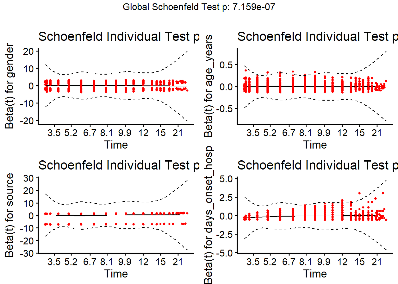

The model results indicate there is a negative association between onset to admission duration and all-cause mortality. The expected hazard is 0.9 times lower in a person who who is one day later admitted than another, holding gender constant. Or in a more straightforward explanation, a one unit increase in the duration of onset to admission is associated with a 10.7% (coef *100) decrease in the risk of death.

Results show also a positive association between the source of infection and the all-cause mortality. Which is to say there is an increased risk of death (1.21x) for patients that got a source of infection other than funerals.

#print the summary of the model
summary(linelistsurv_cox)

## Call:
## coxph(formula = Surv(futime, event) ~ gender + age_years + source + 
##     days_onset_hosp, data = linelist_surv)
## 
##   n= 2772, number of events= 1180 
##    (1767 observations deleted due to missingness)
## 
##                      coef exp(coef)  se(coef)      z Pr(>|z|)    
## genderm          0.004710  1.004721  0.060827  0.077   0.9383    
## age_years       -0.002249  0.997753  0.002421 -0.929   0.3528    
## sourceother      0.178393  1.195295  0.084291  2.116   0.0343 *  
## days_onset_hosp -0.104063  0.901169  0.014245 -7.305 2.77e-13 ***
## ---
## Signif. codes:  0 '***' 0.001 '**' 0.01 '*' 0.05 '.' 0.1 ' ' 1
## 
##                 exp(coef) exp(-coef) lower .95 upper .95
## genderm            1.0047     0.9953    0.8918    1.1319
## age_years          0.9978     1.0023    0.9930    1.0025
## sourceother        1.1953     0.8366    1.0133    1.4100
## days_onset_hosp    0.9012     1.1097    0.8764    0.9267
## 
## Concordance= 0.566  (se = 0.009 )
## Likelihood ratio test= 71.31  on 4 df,   p=1e-14
## Wald test            = 59.22  on 4 df,   p=4e-12
## Score (logrank) test = 59.54  on 4 df,   p=4e-12

We can verify this relationship with a table:

linelist_case_data %>% 
  tabyl(days_onset_hosp, outcome) %>% 
  adorn_percentages() %>%  
  adorn_pct_formatting()

##  days_onset_hosp Death Recover   NA_
##                0 44.3%   31.4% 24.3%
##                1 46.6%   32.2% 21.2%
##                2 43.0%   32.8% 24.2%
##                3 45.0%   32.3% 22.7%
##                4 41.5%   38.3% 20.2%
##                5 40.0%   36.2% 23.8%
##                6 32.2%   48.7% 19.1%
##                7 31.8%   38.6% 29.5%
##                8 29.8%   38.6% 31.6%
##                9 30.3%   51.5% 18.2%
##               10 16.7%   58.3% 25.0%
##               11 36.4%   45.5% 18.2%
##               12 18.8%   62.5% 18.8%
##               13 10.0%   60.0% 30.0%
##               14 10.0%   50.0% 40.0%
##               15 28.6%   42.9% 28.6%
##               16 20.0%   80.0%  0.0%
##               17  0.0%  100.0%  0.0%
##               18  0.0%  100.0%  0.0%
##               22  0.0%  100.0%  0.0%
##               NA 52.7%   31.2% 16.0%

We would need to consider and investigate why this association exists in the data. One possible explanation could be that patients who live long enough to be admitted later had less severe disease to begin with. Another perhaps more likely explanation is that since we used a simulated fake dataset, this pattern does not reflect reality!

Forest plots

We can then visualize the results of the cox model using the practical forest plots with the ggforest() function of the survminer package.

ggforest(linelistsurv_cox, data = linelist_surv)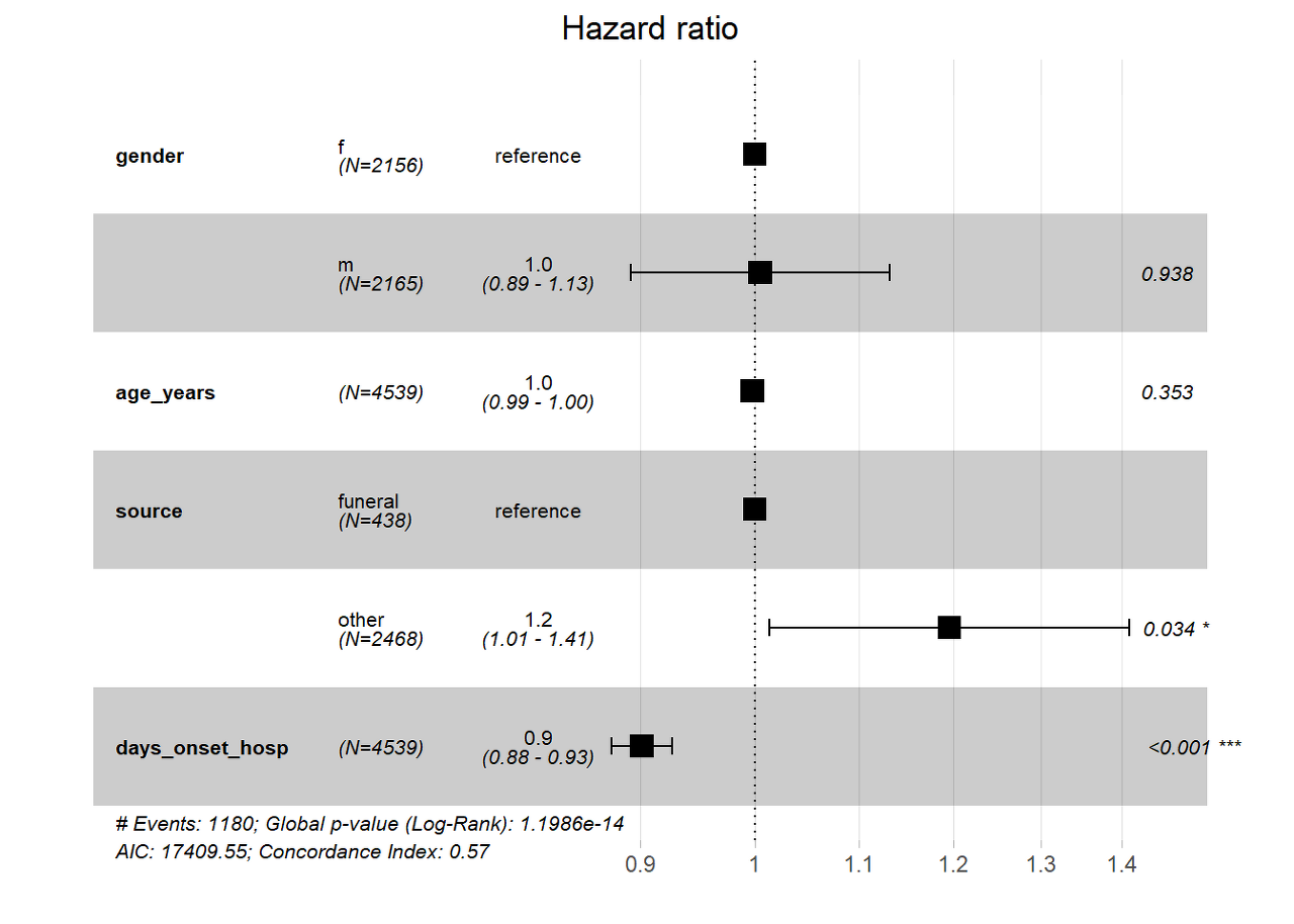

27.6 Time-dependent covariates in survival models

Some of the following sections have been adapted with permission from an excellent introduction to survival analysis in R by Dr. Emily Zabor

In the last section we covered using Cox regression to examine associations between covariates of interest and survival outcomes.But these analyses rely on the covariate being measured at baseline, that is, before follow-up time for the event begins.

What happens if you are interested in a covariate that is measured after follow-up time begins? Or, what if you have a covariate that can change over time?

For example, maybe you are working with clinical data where you repeated measures of hospital laboratory values that can change over time. This is an example of a Time Dependent Covariate. In order to address this you need a special setup, but fortunately the cox model is very flexible and this type of data can also be modeled with tools from the survival package.

Time-dependent covariate setup

Analysis of time-dependent covariates in R requires setup of a special dataset. If interested, see the more detailed paper on this by the author of the survival package Using Time Dependent Covariates and Time Dependent Coefficients in the Cox Model.

For this, we’ll use a new dataset from the SemiCompRisks package named BMT, which includes data on 137 bone marrow transplant patients. The variables we’ll focus on are:

T1 - time (in days) to death or last follow-up
delta1 - death indicator; 1-Dead, 0-Alive
TA - time (in days) to acute graft-versus-host disease
deltaA - acute graft-versus-host disease indicator;
- 1 - Developed acute graft-versus-host disease
- 0 - Never developed acute graft-versus-host disease

We’ll load this dataset from the survival package using the base R command data(), which can be used for loading data that is already included in a R package that is loaded. The data frame BMT will appear in your R environment.

data(BMT, package = "SemiCompRisks")

Add unique patient identifier

There is no unique ID column in the BMT data, which is needed to create the type of dataset we want. So we use the function rowid_to_column() from the tidyverse package tibble to create a new id column called my_id (adds column at start of data frame with sequential row ids, starting at 1). We name the data frame bmt.

bmt <- rowid_to_column(BMT, "my_id")

The dataset now looks like this:

Show

entries

Search:

my_idgT1T2delta1delta2delta3TAdeltaATCdeltaCTPdeltaPZ1Z2Z3Z4Z5Z6Z7Z8Z9Z10

1	1	2081	2081	67	1	121	1	13	1	26	33	1	0	1	1	98	1
2	1	1602	1602	1602	0	139	1	18	1	21	37	1	1	0	0	1720	1
3	1	1496	1496	1496	0	307	1	12	1	26	35	1	1	1	0	127	1
4	1	1462	1462	70	1	95	1	13	1	17	21	0	1	0	0	168	1
5	1	1433	1433	1433	0	236	1	12	1	32	36	1	1	1	1	93	1

Showing 1 to 5 of 137 entries

Previous1 2 3 4 5…28Next

Expand patient rows

Next, we’ll use the tmerge() function with the event() and tdc() helper functions to create the restructured dataset. Our goal is to restructure the dataset to create a separate row for each patient for each time interval where they have a different value for deltaA. In this case, each patient can have at most two rows depending on whether they developed acute graft-versus-host disease during the data collection period. We’ll call our new indicator for the development of acute graft-versus-host disease agvhd.

tmerge() creates a long dataset with multiple time intervals for the different covariate values for each patient
event() creates the new event indicator to go with the newly-created time intervals
tdc() creates the time-dependent covariate column, agvhd, to go with the newly created time intervals

td_dat <- 
  tmerge(
    data1 = bmt %>% select(my_id, T1, delta1), 
    data2 = bmt %>% select(my_id, T1, delta1, TA, deltaA), 
    id = my_id, 
    death = event(T1, delta1),
    agvhd = tdc(TA)
    )

To see what this does, let’s look at the data for the first 5 individual patients.

The variables of interest in the original data looked like this:

bmt %>% 
  select(my_id, T1, delta1, TA, deltaA) %>% 
  filter(my_id %in% seq(1, 5))

##   my_id   T1 delta1   TA deltaA
## 1     1 2081      0   67      1
## 2     2 1602      0 1602      0
## 3     3 1496      0 1496      0
## 4     4 1462      0   70      1
## 5     5 1433      0 1433      0

The new dataset for these same patients looks like this:

td_dat %>% 
  filter(my_id %in% seq(1, 5))

##   my_id   T1 delta1 tstart tstop death agvhd
## 1     1 2081      0      0    67     0     0
## 2     1 2081      0     67  2081     0     1
## 3     2 1602      0      0  1602     0     0
## 4     3 1496      0      0  1496     0     0
## 5     4 1462      0      0    70     0     0
## 6     4 1462      0     70  1462     0     1
## 7     5 1433      0      0  1433     0     0

Now some of our patients have two rows in the dataset corresponding to intervals where they have a different value of our new variable, agvhd. For example, Patient 1 now has two rows with a agvhd value of zero from time 0 to time 67, and a value of 1 from time 67 to time 2081.

Cox regression with time-dependent covariates

Now that we’ve reshaped our data and added the new time-dependent aghvd variable, let’s fit a simple single variable cox regression model. We can use the same coxph() function as before, we just need to change our Surv() function to specify both the start and stop time for each interval using the time1 = and time2 = arguments.

bmt_td_model = coxph(
  Surv(time = tstart, time2 = tstop, event = death) ~ agvhd, 
  data = td_dat
  )

summary(bmt_td_model)

## Call:
## coxph(formula = Surv(time = tstart, time2 = tstop, event = death) ~ 
##     agvhd, data = td_dat)
## 
##   n= 163, number of events= 80 
## 
##         coef exp(coef) se(coef)    z Pr(>|z|)
## agvhd 0.3351    1.3980   0.2815 1.19    0.234
## 
##       exp(coef) exp(-coef) lower .95 upper .95
## agvhd     1.398     0.7153    0.8052     2.427
## 
## Concordance= 0.535  (se = 0.024 )
## Likelihood ratio test= 1.33  on 1 df,   p=0.2
## Wald test            = 1.42  on 1 df,   p=0.2
## Score (logrank) test = 1.43  on 1 df,   p=0.2

Again, we’ll visualize our cox model results using the ggforest() function from the survminer package.:

ggforest(bmt_td_model, data = td_dat)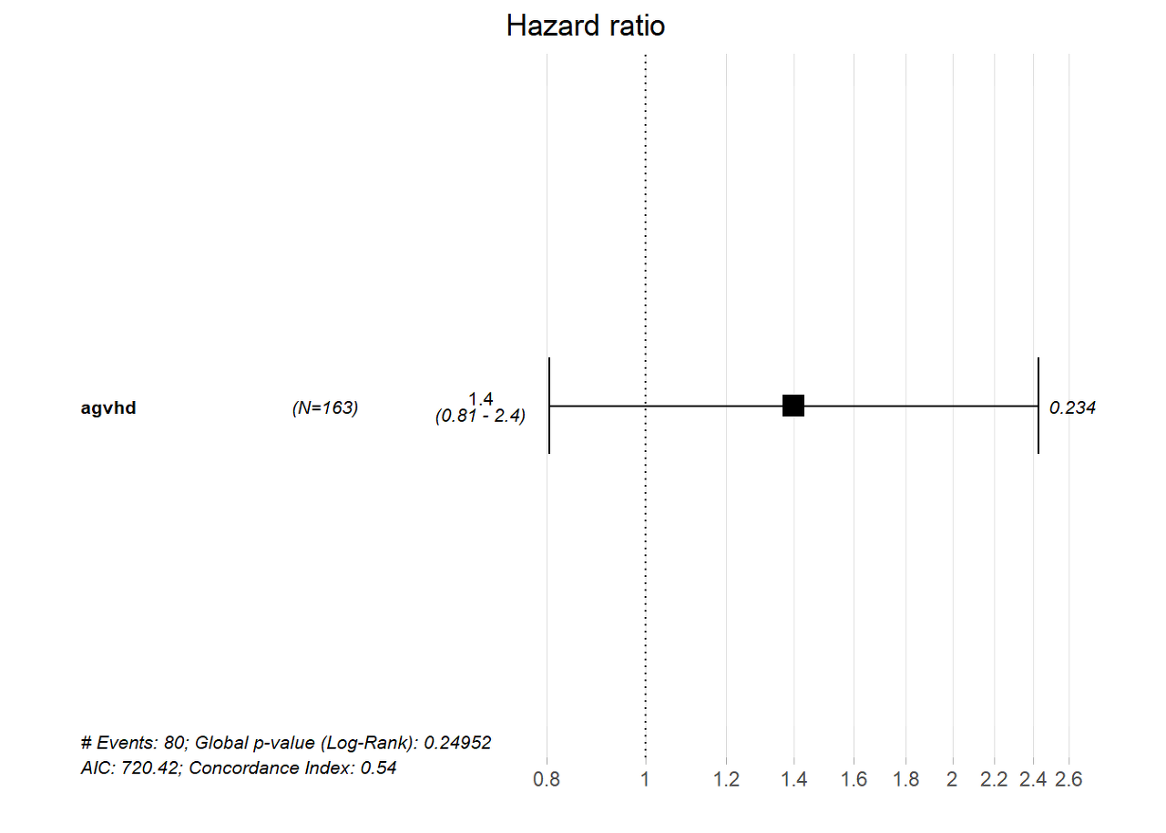

As you can see from the forest plot, confidence interval, and p-value, there does not appear to be a strong association between death and acute graft-versus-host disease in the context of our simple model.